40 pole zero diagram matlab

Pole Zero Plot of Transfer Fucntion H(z). Learn more about pole ... How can i have its pole zero map ... Isn't that the poles and zeros already given?2 answers · 0 votes: is it good approach. i have actual H(z) in z(-1) form h = tf([1 -1],[1 -3 2],0.1,'variable','z^-1') ... http://adampanagos.orgA Matlab script is used to design a variety of different digital filters. This is accomplished by placing poles in and zeros in the Z-...

I need to do two things with this using MATLAB: Find it's z -transform. Plot it's poles and zeros. I am using the following code: syms n; f = (1/2)^n + (-1/3)^n; F = ztrans (f); I get the z -transform in the F variable, but I can't see how to create it's pole-zero plot. I am using the built-in function pzmap ( pzmap (F); ), but it doesn't seem ...

Pole zero diagram matlab

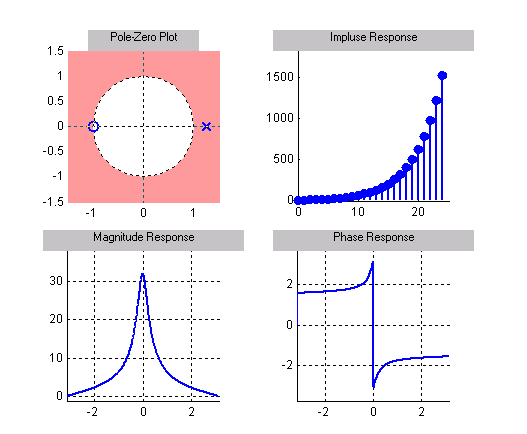
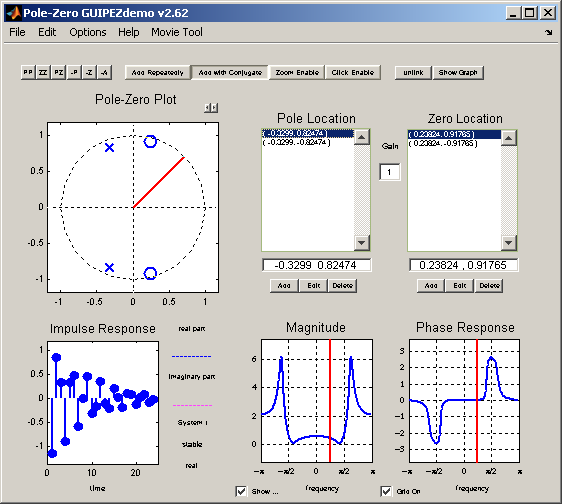
Click "Add pole" or "Add zero". Move the pole/zero around the plane. Observe the change in the magnitude and phase Bode plots. Info: Only the first (green) transfer function is configurable. Blue and red transfer functions are cleared when moving poles/zeroes in the plane. Scenario: 1 pole/zero: can be on real-axis only Pole-Zero Analysis This chapter discusses pole-zero analysis of digital filters.Every digital filter can be specified by its poles and zeros (together with a gain factor). Poles and zeros give useful insights into a filter's response, and can be used as the basis for digital filter design.This chapter additionally presents the Durbin step-down recursion for checking filter stability by finding ... Pole Zero Diagram. pole-zero plot in mathematics signal processing and control theory a pole-zero plot is a graphical representation of a rational transfer function in the plex plane understanding poles and zeros 1 system poles and … - mit massachusetts institute of technology department of mechanical engineering 2 14 analysis and design of feedback control systems understanding poles ...

Pole zero diagram matlab. The following plot shows the transient response of a system with a real zero and a pair of complex poles for a unit-impulse input and a unit-step input. The response of the system without the zero is also included for comparison. The poles and zero can be dragged on the s-plane to see the effect on the response. zplane(z,p) plots the zeros specified in column vector z and the poles specified in column vector p in the current figure window.The symbol 'o' represents a zero and the symbol 'x' represents a pole. The plot includes the unit circle for reference. If z and p are matrices, then zplane plots the poles and zeros in the columns of z and p in different colors. zplane(z,p) plots the zeros specified in column vector z and the poles specified in column vector p in the current figure window.The symbol 'o' represents a zero and the symbol 'x' represents a pole. The plot includes the unit circle for reference. If z and p are matrices, then zplane plots the poles and zeros in the columns of z and p in different colors. pzmap (sys1,sys2,...,sysN) creates the pole-zero plot of multiple models on a single figure. The models can have different numbers of inputs and outputs and can be a mix of continuous and discrete systems. For SISO systems, pzmap plots the system poles and zeros. For MIMO systems, pzmap plots the system poles and transmission zeros.

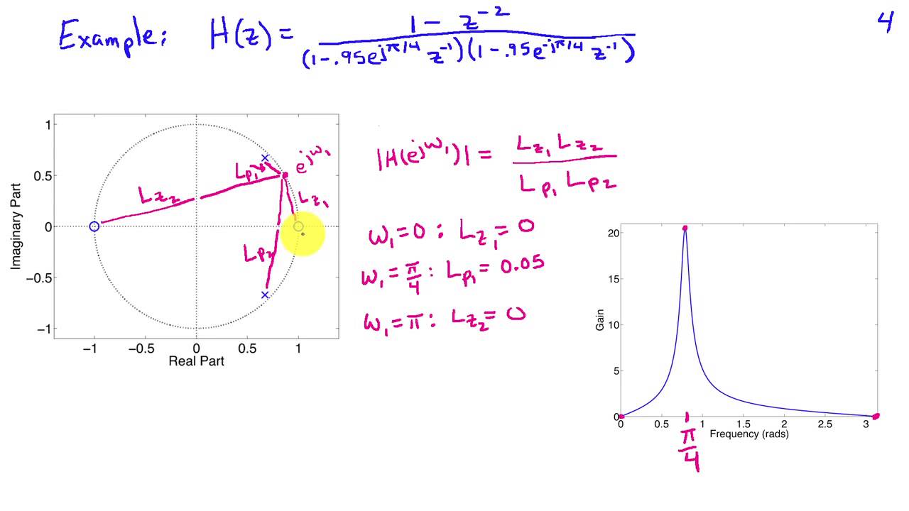
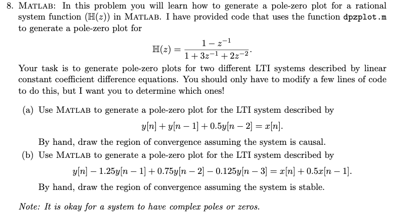
Pole Zero Plot of Transfer Fucntion H(z). Learn more about pole Control System Toolbox pzmap (sys1,sys2,...,sysN) creates the pole-zero plot of multiple models on a single figure. The models can have different numbers of inputs and outputs and can be a mix of continuous and discrete systems. For SISO systems, pzmap plots the system poles and zeros. For MIMO systems, pzmap plots the system poles and transmission zeros. example. Science; Advanced Physics; Advanced Physics questions and answers; Question 1 A causal LTI system has the following system function H(-) = (1 - 4j7/3,-1)(1 - e-ja/3.-1)(1+ (1/0.85)2-1) (1 - 0.9ejn/3,-1)(1 - .9e-ja/3,-1)(1+0.852-1) (a) Expand the impulse response and plot the pole-zero diagram using Matlab's zplane function and indicate the region of convergence for the system function. MATLAB - If access to MATLAB is readily available, then you can use its functions to easily create pole/zero plots. Below is a short program that plots the poles and zeros from the above example onto the Z-Plane.

Plot the pole-zero map of a discrete time identified state-space (idss) model. In practice you can obtain an idss model by estimation based on input-output measurements of a system. For this example, create one from state-space data. You can create a pole-zero plot for linear identified models using the iopzmap and iopzplot commands. Bode diagram design is an interactive graphical method of modifying a compensator to achieve a specific open-loop response. ... At the MATLAB ® command line ... the app updates the pole/zero values and updates the response plots. To decrease the magnitude of a pole or zero, drag it towards the left. ... Click the Pole/Zero Plot toolbar button, select Analysis > Pole/Zero Plot from the menu, or type the following code to see the plot. fvtool(b,a, 'Analysis', 'polezero') ... You clicked a link that corresponds to this MATLAB command: Run the command by entering it in the MATLAB Command Window.

Hi, U can get the poles and zeros by using the command. tf2zp (transfer to pole zero). check this out u will find a quick solution. regds,sree. "satnam74 <>" <> wrote:hi, I want to get the pole zero diagram for y as given below. Can. anybody in the group help me please.

This MATLAB function computes and plots the poles and zeros of each ...

Plot pole-zero diagram for a given tran... How to make GUI | Part 2 | MATLAB Guide | MATLAB Tutorial How to make GUI with MATLAB Guide Part 2 - MATLAB Tutorial (MAT & CAD Tips) This Video is the next part of the previous video.

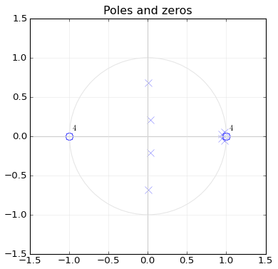
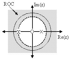
Zero-Pole Analysis. The zplane function plots poles and zeros of a linear system. For example, a simple filter with a zero at -1/2 and a complex pole pair at 0. 9 e - j 2 π 0. 3 and 0. 9 e j 2 π 0. 3 is. To view the pole-zero plot for this filter you can use zplane. Supply column vector arguments when the system is in pole-zero form.

Dengan MatLab gambarlah pole-zero plot dari sistem seperti pada soal 2. Soal 7. Dengan MatLab gambarlah Bode plot dari sistem dengan transfer function: H(s)=a/(s 2 +s+b). Soal 8. Dari gambar Bode plot pada soal 7 tentukan gain sistem untuk frekuensi a rad/det. ...

What Does a Pole-Zero Plot Show? — You can create pole-zero plots of linear identified models. To study the poles and zeros of the noise component of ...

Based on the transfer function, the poles and zeros can be defined as, a = [1 -2.2343 1.8758 -0.5713] b = [0.0088 0.0263 0.0263 0.0088] This is where my confusion starts. based on the first tutorial, i'll have to plot all the zeros/poles along the x-axis (Or am I mistaken?). But based on the MATLAB command to plot pole and zeros, zplane (a,b) I ...

Pole-Zero Plot with Custom Plot Title — pzplot lets you plot pole-zero maps with a broader range of plot customization options than pzmap .

MATLAB ® FUNCTIONS ZPK Create zero-pole-gain models or convert to zero-pole-gain format. Creation: SYS = ZPK(Z,P,K) creates a continuous-time zero-pole-gain (ZPK) model SYS with zeros Z, poles P, and gains K. The output SYS is a ZPK object. SYS = ZPK(Z,P,K,Ts) creates a discrete-time ZPK model with sample

pzplot lets you plot pole-zero maps with a broader range of plot customization options than pzmap.You can use pzplot to obtain the plot handle and use it to customize the plot, such as modify the axes labels, limits and units. You can also use pzplot to draw a pole-zero plot on an existing set of axes represented by an axes handle.

pzplot plots pole and zero locations on the complex plane as x and o marks, respectively. When you provide multiple models, pzplot plots the poles and zeros of each model in a different color. Here, there poles and zeros of CL1 are blue, and those of CL2 are green.. The plot shows that all poles of CL1 are in the left half-plane, and therefore CL1 is stable. . From the radial grid markings on ...

Root locus design is a common control system design technique in which you edit the compensator gain, poles, and zeros in the root locus diagram. As the open-loop gain, k, of a control system varies over a continuous range of values, the root locus diagram shows the trajectories of the closed-loop poles of the feedback system.

About Press Copyright Contact us Creators Advertise Developers Terms Privacy Policy & Safety How YouTube works Test new features Press Copyright Contact us Creators ...

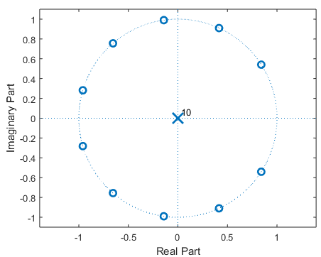
Figure 1: The pole-zero plot for a typical third-order system with one real pole and a complex conjugate pole pair, and a single real zero. 1.1 The Pole-Zero Plot A system is characterized by its poles and zeros in the sense that they allow reconstruction of the input/output diﬀerential equation.

Pole-Zero Plot with Custom Options — Use the pzoptions command to create a PZMapOptions object to customize your pole/zero plot appearance. You can ...

In addition, preset pole-zero diagrams (in fact, all-pole systems) for vowels can be loaded. Note: this demonstration requires the Matlab Signal Processing Toolbox. The tool. Type 'polezero' to launch the demo. You will be presented with a display dominated by the unit circle. Initially, it contains no poles or zeroes.

Entering the following commands into the MATLAB command window will generate the following output. zeros = zero (C*P_pend) poles = pole (C*P_pend) zeros = 0 poles = 0 5.5651 -5.6041 -0.1428. As you can see, there are four poles and only one zero. This means that the root locus will have three asymptotes: one along the real axis in the negative ...

Pole Zero Diagram. pole-zero plot in mathematics signal processing and control theory a pole-zero plot is a graphical representation of a rational transfer function in the plex plane understanding poles and zeros 1 system poles and … - mit massachusetts institute of technology department of mechanical engineering 2 14 analysis and design of feedback control systems understanding poles ...

Pole-Zero Analysis This chapter discusses pole-zero analysis of digital filters.Every digital filter can be specified by its poles and zeros (together with a gain factor). Poles and zeros give useful insights into a filter's response, and can be used as the basis for digital filter design.This chapter additionally presents the Durbin step-down recursion for checking filter stability by finding ...